CS 184 Final Project: Going Sigma on ViCMA (GSV)

Bill Shao, Jonathan Pei, Tobias Worledge, Dominic Conricode

Website: https://jonnypei.github.io/illusion-sim-website/final/index.html

Video: https://tinyurl.com/sigma-vicma-video


Abstract


In this project, we replicate and extend ViCMA (Visual Control of Multibody Animations), a visual control method that exploits object motion and visibility to manipulate shading during an animation sequence. For replication, we used blender to construct simulations and built off of our cloth simulation code to implement the ViCMA shading control. In doing so, we modify the rendering pipeline to support polyhedral structures, generalized spatial hashing, and per-object texture mapping. For extensions, we add support for gradient color transitions (as opposed to single-frame flips) and modify the ViCMA heuristic to include color locality (beyond just the position and velocity localities). Our full code implementation is available at the following github repo: https://github.com/jonnypei/illusion-sim.


Technical Approaches

For our technical approaches, we implemented the following:
  1. Custom Blender to ViCMA Simulation Pipeline.
  2. Modifications to Cloth Simulation Rendering Pipeline.
  3. ViCMA Code Implementation.
  4. Gradient Transitions for ViCMA.

(1) Blender to ViCMA Simulation Pipeline

Overview:

Rather than implement our own rigidbody simulator for ViCMA, we instead took advantage of Blender's built-in rigidbody physics simulator. We made this decision to simplify the physical processing required when creating simulations to "ViCMA-ify".

Part 1: Blender Simulation Environment

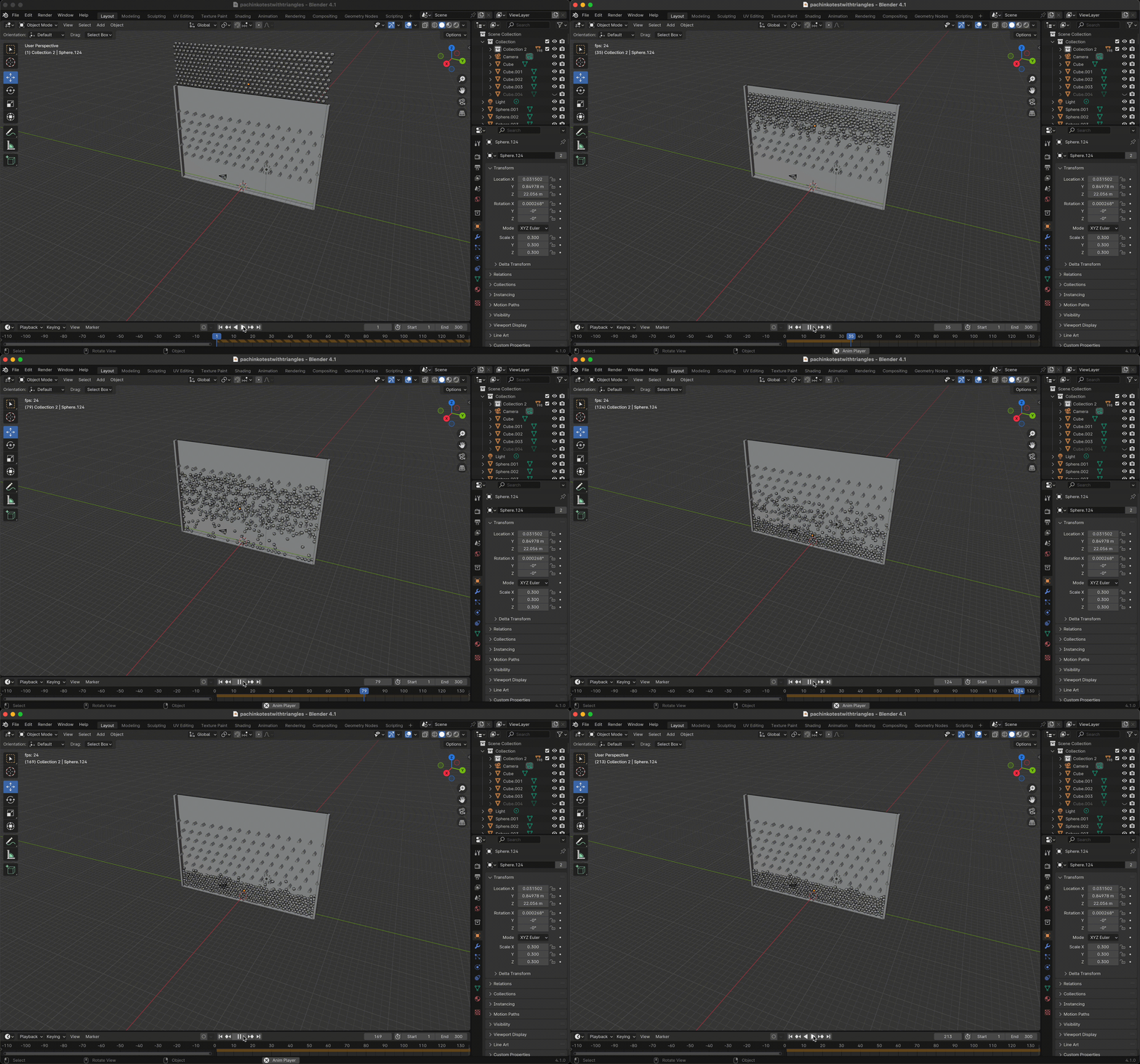
Our first step to create a new simulation is to generate the scene in Blender. We did this by first organizing all scene objects, then applying Blender's built-in rigidbody property. Below is an example for pachinkotestwithtriangles.

Part 2: Blender Export Data Structure

After fully rendering the scene in Blender, we needed to import the position and rotation data for each object at every timestep into our ViCMA Simulator. We were ultimately able to do this using Blender's scripting API bpy. The script generates two important resources, a custom scene.json and a set of anim_files for each object.

scene.json

The scene.json contains initialization parameters for both static and dynamic objects in the scene and records their starting location, color settings, and render parameters for non-spherical meshes. Below is an example of a random entry in scene.json.
    "Sphere.001": {
      "start_color": 
      [0.75,0.26,1,0.9],
      "end_color": 
      [0.3,1,0,0.9],
      "origin": 
      [-8.361442565917969,26.15984535217285,29.98017120361328],
      "radius": 1
    }
    

anim_files

anim_files is a folder containing files labeled scene_name/object_name.txt which records position data of a dynamic object at each frame of the simulation. In each file, every three entries cooresponds to one (x,y,z) position.

Interesting Debugging:

While implementing the export script for dynamic objects, we had an issue where the item.location paramater for each object would not change. Upon debugging, we realized this was due to Blender using a similar object-world space as described in the translations lecture. Thus, we were exporting out the positions in object space, which didn't change throughout the animation. To resolve this, we first found the object2world matrix and multiplied it with the object space vector to get the final world space vector.

    v = item.data.vertices[vertex_ind].co
    mat = item.matrix_world
    v = mat @ v
    

Part 3: ViCMA Simulator Loading Pipeline

AnimationObject struct

To load the exported scene.json and anim_files into the simulator, we first created a new set set of AnimationObject structures that could load in and process the extra data. Two structs, Spheres and Polygons, were implemented to handle this task. Below are some notable object parameters and functions that were implemented for each of these classes in the simulator.
    int curr_frame;
    int start_transition_frame;
    vector<Vector3D> positions;
    vector<Vector3D> velocities;
    nanogui::Color start_color;
    nanogui::Color curr_color;
    nanogui::Color end_color;
    shape objShape;
    string name;

    void render(GLShader &shader);
    void simulate();
    void reset();
    
The process of simulating AnimationObjects was simple, and consisted of updating the curr_frame parameter. The render() function would then use curr_frame to update the position of the rendered object based on positions.

Object Parser

The parsing of json files and anim_files was handled by modifications to loadObjectsFromFile. Basic key-switch operations were added to include the new polygons, and we also implemented the readFileAndGetPosVec function to convert each anim_file into vector<Vector3D> positions.

Example of Simplicity in Pipeline

Below, we provide an example demonstrating the simplicity of using our pipeline.

(2) Modifications to Cloth Simulation Rendering Pipeline

To setup the codebase for ViCMA implementation, we made the following modifications to the original cloth simulation pipeline:
  1. Built new rendering function for polygons; see below for our implementation:
  2.     void AnimationObject::renderPoly(GLShader &shader) {
          Matrix4f model;
          model << 1, 0, 0, 0, 0, 1, 0, 0, 0, 0, 1, 0, 0, 0, 0, 1;
          shader.setUniform("u_model", model);
    
          Vector3D centroid = Vector3D(0, 0, 0);
          vector scaled_vertices;
          for (auto &vertex : vertices) {
            centroid += vertex;
          }
          centroid /= vertices.size();
          for (auto &vertex : vertices) {
            scaled_vertices.push_back((vertex - centroid) * 1 + centroid);
          }
    
          for (auto &face : faces) {
            MatrixXf positions(3, face.size());
            MatrixXf normals(3, face.size());
    
            for (int i = 0; i < face.size(); i++) {
              positions.col(i) << scaled_vertices[face[i]].x,
                  scaled_vertices[face[i]].y, scaled_vertices[face[i]].z;
              normals.col(i) << vertex_normals[face[i]].x, vertex_normals[face[i]].y,
                  -vertex_normals[face[i]].z;
            }
    
            if (shader.uniform("u_color", false) != -1) {
              shader.setUniform("u_color", this->curr_color);
            }
            shader.uploadAttrib("in_position", positions);
            if (shader.attrib("in_normal", false) != -1) {
              shader.uploadAttrib("in_normal", normals);
            }
    
            shader.drawArray(GL_TRIANGLE_FAN, 0, face.size());
          }
        }
        
  3. Incorporated spatial hashing for the ViCMA spatial neighborhood computation.
  4. Implemented per-object texturing by adding separate shaders for each object in clothSimulator.cpp, mainly writing logic in ClothSimulator::drawContents().
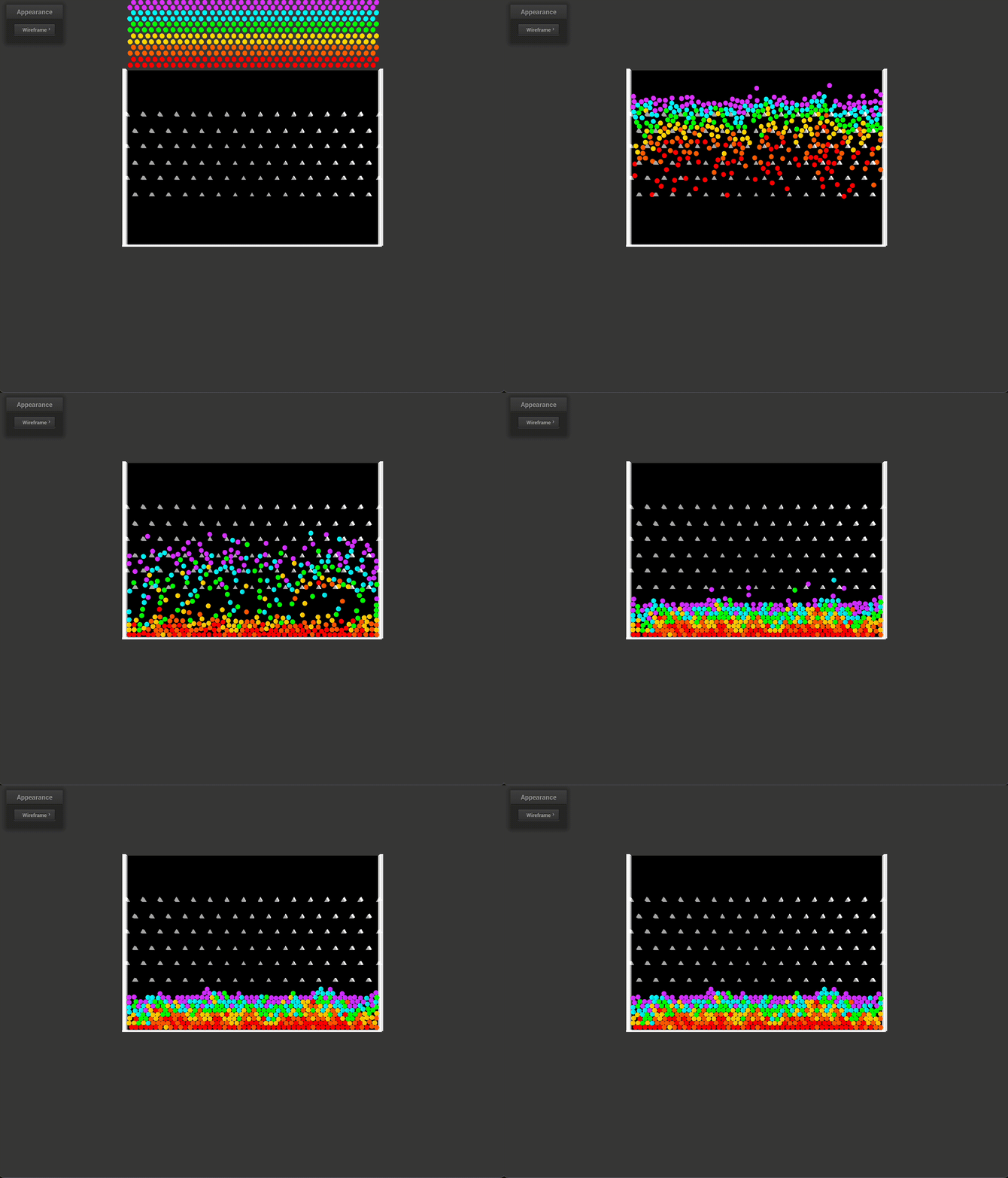
  5. Built an pipeline for light scene creation; this was mainly used to experiment with the various shading implemented in the original Cloth Simulator.

(3) ViCMA Theory and Implementation

Overview

ViCMA is a visual control method for passive multibody systems, exploiting visual perception and attention for purely appearance-based control (as opposed to physically-based). In particular, given a set of keyframes for a multibody animation with a start/end appearance for all objects, ViCMA computes the optimal appearance transition keyframe for every object. To do this, ViCMA computes a heuristic transition cost \(\phi_i^{vicma}\) for each object \(i\) in every frame, and valid appearance transition keyframes for each object are those with minimal cost.

A crucial property of this heuristic is that it is local (i.e. only relies on given object and spatial neighborhood), enabling fast computation and simple parallelization. As such, we compute the ViCMA transition frames when loading in the Blender scene .json files in main.cpp. Then, during rendering, we simply perform an appearance change for a given object at its transition frame.

The ViCMA heuristic consists of 2 main cost types: visibility cost \(\phi_i^{viz}\) and motion cost \(\phi_i^{motion}\).

Visibility Cost

ViCMA exploits the visibility changes to transition objects when they are out of sight, or have low projected area in the frame. Thus, it contains a visibility cost defined as the average projected area of an object onto the scene, computed from rasterized object ID images. For each object \(i\), we compute $$\phi_i^{viz} = \frac{1}{N_{pixels}} \sum_{j,k=1}^{N_{pixels}} \mathbf{1}\{\text{ID}_i == \text{ID}(j, k)\},$$ where \(N_{pixels}\) is the number of pixels in the ID images of object \(i\), \(\text{ID}_i\) is the ID for object \(i\), and \(\text{ID}(j, k)\) is the ID stored at pixel \((j, k)\) in the ID image.

Motion Cost

For scenes in which we cannot exploit visibility changes as much (e.g. where objects are always visible), ViCMA incorporates a multipart motion cost to exploit the chaotic nature of motion and mixing for concealing appearance changes.

First, ViCMA defines a velocity-level heuristic that penalizes changes for objects at rest, and awards changes for objects moving near fast surrounding objects: $$\phi_i^{vel} = \exp\left[-\left(\frac{\min(v_i, \sigma_i)}{\delta v}\right)^2\right] \in [0, 1].$$ Here, \(v_i = \|\mathbf{v}_i\|\) denotes the speed of object \(i\) traveling at velocity \(\mathbf{v}_i\), and \(\delta v\) is a user-defined scaling parameter. \(\sigma_i\) is defined as the velocity standard deviation of surrounding objects: $$\sigma_i^2 = \frac{1}{\mathcal{N}_i} \sum_{j \in \mathcal{N}_i} \|\bar{\mathbf{v}}_i - \mathbf{v}_j\|^2 \quad \text{with} \quad \bar{\mathbf{v}}_i = \frac{1}{\mathcal{N}_i} \sum_{j \in \mathcal{N}_i} \mathbf{v}_j,$$ where \(\mathcal{N}_i\) is the set of neighboring objects with centroids within a spatial distance of \(R_i = 4r_i\). Note that \(r_i\) is the bounding radius of object \(i\).

An issue with \(\phi_i^{vel}\) above is that it can create transitions where a single fast-moving object hits a stationary object, causing it to change appearance in an obvious manner. To discourage this, ViCMA uses a movement-level heuristic to award more moving neighbors by explicitly counting: $$\phi_i^{mov} = 1 - \text{smooth}(n_{min}, n_{max}, n_i^{mov}),$$ where we apply the cubic smoothstep function to \(n_{min} = 3, n_{max} = 5\), and \(n_i^{mov}\) (defined below). $$n_i^{mov} = \sum_{j \in \mathcal{N}_i} \mathbf{1}\{\min(v_i, \|\mathbf{v}_i - \mathbf{v}_j\|) > \delta v\}$$

Finally, an issue with both \(\phi_i^{vel}\) and \(\phi_i^{mov}\) above is that they can both be low during early impacts/shockwaves, which can cause a closely packed arrangement of objects to suddenly change appearances before much movement has even occurred. Hence, ViCMA introduces a mixing-level heuristic to discourage transitions from occurring before sufficient spatial mixing. To do this, they devised a directional overlap coefficient to measure the spatial mixture levels of any given frame \((t)\) with respect to the starting \((0)\) and ending \((F)\) frames. $$D_i^{0t} = \frac{1}{|\mathcal{N}_i^0|} \sum_{j \in \mathcal{N}_i^0 \cap \mathcal{N}_i^t} \left(\hat{\mathbf{d}}_{ji}^0 \cdot \hat{\mathbf{d}}_{ji}^t \right)_+, \quad D_i^{Ft} = \frac{1}{|\mathcal{N}_i^F|} \sum_{j \in \mathcal{N}_i^F \cap \mathcal{N}_i^t} \left(\hat{\mathbf{d}}_{ji}^F \cdot \hat{\mathbf{d}}_{ji}^t \right)_+,$$ where \(\hat{\mathbf{d}}_{ji}\) are the normalized displacement vectors from objects \(i\) to \(j\): \(\hat{\mathbf{d}}_{ji} = \frac{\mathbf{x}_j - \mathbf{x}_i}{\|\mathbf{x}_j - \mathbf{x}_i\|}.\) The overall neighborhood mixing cost at frame \(t\) is then defined as: $$\phi_i^{mix} = \max(D_i^{0t}, D_i^{Ft}),$$ which is always 1 at the start and end frames, and zero for isolated particles.

Putting everything together, the overall motion cost for object \(i\) is: $$\phi_i^{motion} = \max\left[\phi_i^{mix}, \frac{1}{2}\left(\phi_i^{vel} + \phi_i^{mov}\right)\right].$$ In practice, it may be the case that there is some lone visible object for which \(\phi_i^{motion} = 1\) throughout the entire simulation. For this type of edge case, we regularize via a tiny single-body velocity cost to finally yield: $$\phi_i^{motion} = \max\left[\phi_i^{mix}, \frac{1}{2}\left(\phi_i^{vel} + \phi_i^{mov}\right)\right] + \epsilon_v \phi_i^v,$$ where \(\epsilon_v = 0.001\) and \(\phi_i^v = \exp\left[-(v_i / \delta v)^2\right]\).

Overall ViCMA Transition Cost

The final per-frame ViCMA cost for object \(i\) is: $$\phi_i^{vicma} = \phi_i^{motion} \cdot \phi_i^{viz}.$$ Valid transition times for each object are minimizers of \(\phi_i^{vicma}\), and are computed only once to be used during rendering.

(4) Gradient Transitions

We noticed that single-frame shader transitions were too abrupt and sometimes were possible to detect. More specifically, this was noticable if an observer unfocuses their vision and watches the scene as a whole. To address this, we hypothesized that shader transitions that are interpolated across multiple frames would be less noticable. Thus, we implemented a gradient transition using linear interpolation. Once we determine the frame that minimizes the ViCMA transition cost, we linearly interpolate the color of the ball from the start color to the end color over a set number of frames. This results in a smoother transition between the two colors.

(5) Visualizing ViCMA

To better understand how ViCMA works, we implemented a visualization of the ViCMA heuristic. This visualization shows the ViCMA transition cost for each object in the scene at each frame. The visualization is color-coded, with blue representing high cost and red representing low cost. The visualization is shown below for the pachinko animation.


Results

We provide results below showcasing how ViCMA controls the outcome colors of an animation.

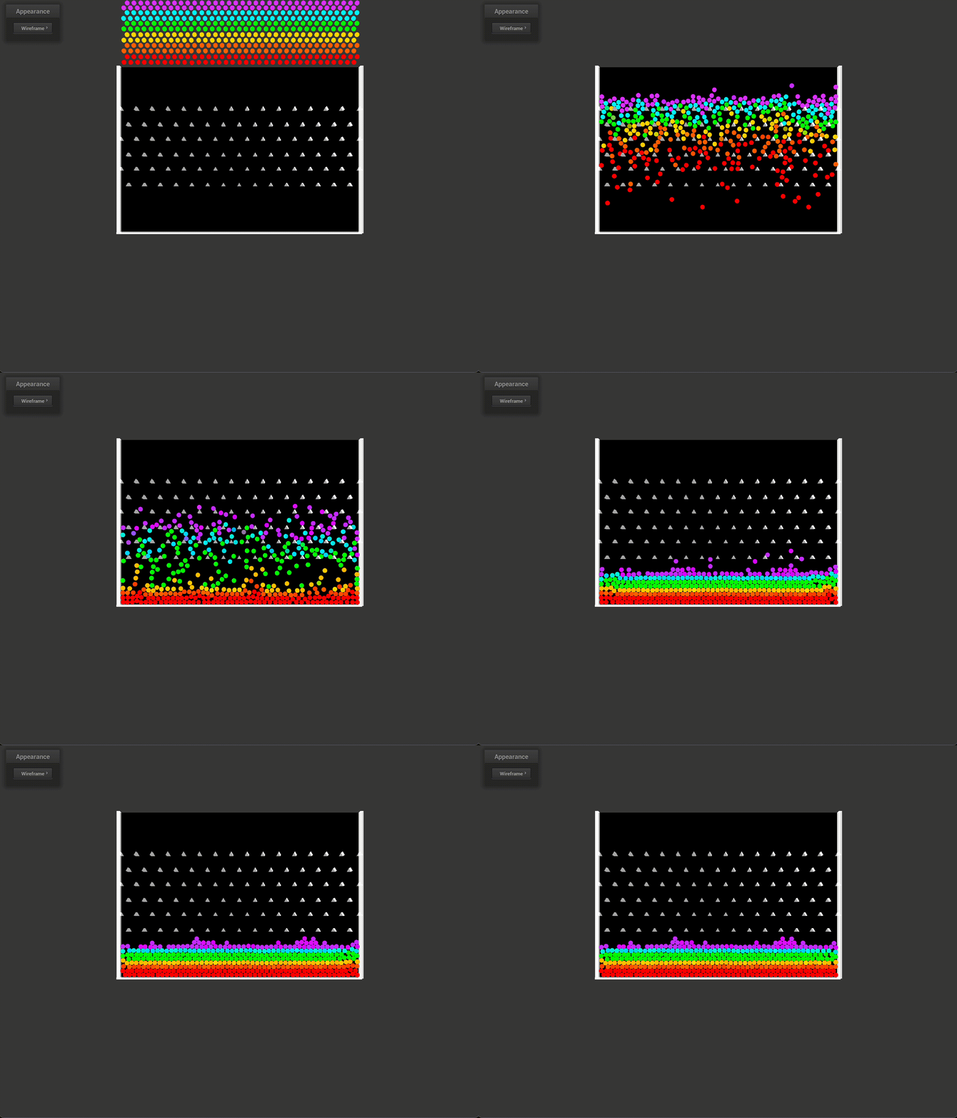
Pachinko Animation without ViCMA
Pachinko Animation with ViCMA
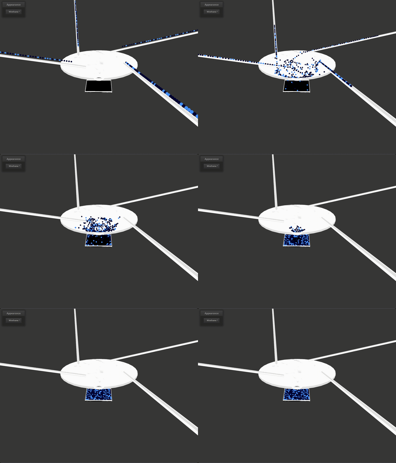
Funnel Animation without ViCMA
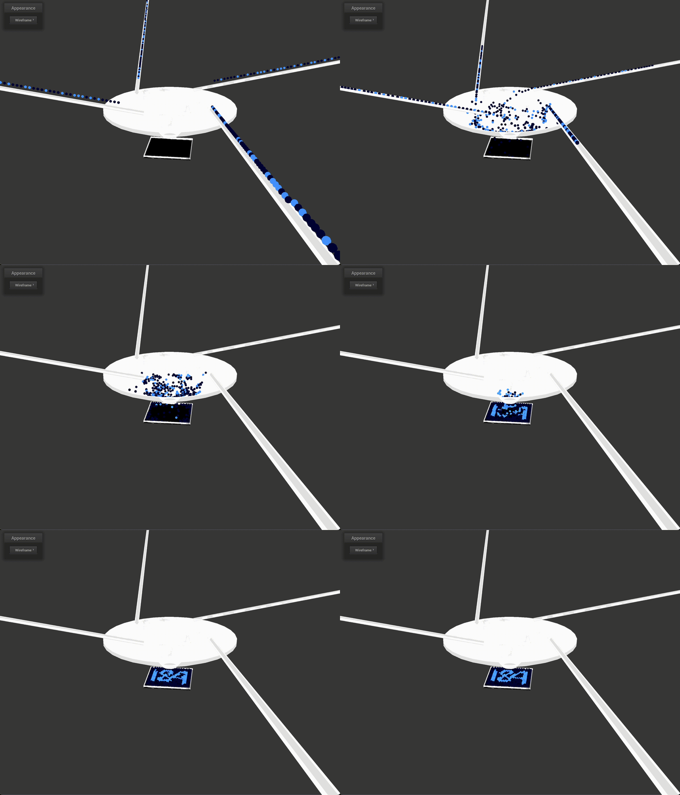
Funnel Animation with ViCMA

We observe that ViCMA is able to effectively control the appearances of the balls in each animation, while making the color transitions almost un-noticeable.

References


Contributions

Bill

Jonny

Toby

Dominic